Naked trading is the best style of trading. Naked trading means trading solely based on price action signals without using any indicators. Just looking at the candlestick signals you can see where the price is going to go. Did you read our post on GBP CPI y/y news trading that made 350+ pips in just 4 hours? Watch the video below that explains how neural networks are being used in trading!
https://www.youtube.com/watch?v=H9Yt5ZmrLzs
In this post we are going to do daily candles predictions using an Elman neural network. Elman neural networks are recurrent neural networks which can be used for financial time series prediction. We download the EURUSD1440.csv from MT4 history center. We hope you know how to download the csv files from MT4 history center. You should have the R and RStudio installed on your computer for doing the required calculations. Let’s start now.
> # Import the csv file
> quotes <- read.csv("E:/MarketData/EURUSD1440.csv", header=FALSE)
> tail(quotes)
             V1    V2      V3      V4      V5      V6     V7
2209 2016.05.20 00:00 1.12027 1.12377 1.11964 1.12185  88486
2210 2016.05.23 00:00 1.12125 1.12430 1.11877 1.12203  93154
2211 2016.05.24 00:00 1.12201 1.12269 1.11324 1.11408 106161
2212 2016.05.25 00:00 1.11394 1.11670 1.11289 1.11552  99307
2213 2016.05.26 00:00 1.11545 1.12169 1.11494 1.11940 105208
2214 2016.05.27 00:00 1.11941 1.12008 1.11111 1.11131  97768
> #number of rows in the dataframe
> x <-nrow(quotes)
>
> # load quantmod package
> library(quantmod)
Loading required package: xts
Loading required package: zoo

Attaching package: ‘zoo’

The following objects are masked from ‘package:base’:

    as.Date, as.Date.numeric

Loading required package: TTR
Version 0.4-0 included new data defaults. See ?getSymbols.
>
> #convert the data frame into a ts object
> quotes <- as.ts(quotes)
>
> #convert time series into a zoo object
> quotes1 <- as.zoo(quotes)
>
>
> # lag the data
> x1 <- lag(quotes1, k=-1, na.pad=TRUE)
> x2 <- lag(quotes1, k=-2, na.pad=TRUE)
> x3 <- lag(quotes1, k=-3, na.pad=TRUE)
> x4 <- lag(quotes1, k=-4, na.pad=TRUE)
> x5 <- lag(quotes1, k=-5, na.pad=TRUE)
> x6 <- lag(quotes1, k=-6, na.pad=TRUE)
> x7 <- lag(quotes1, k=-7, na.pad=TRUE)
> x8 <- lag(quotes1, k=-8, na.pad=TRUE)
> x9 <- lag(quotes1, k=-9, na.pad=TRUE)
> x10 <-lag(quotes1, k=-10, na.pad=TRUE)
>
> #
> #Neural Network for the Close Price Time Series
> #
>
>
> # combine all the above matrices into one matrix having close prices
> CQuotes <- cbind (x1[,6], x2[,6], x3[,6], x4[,6], x5[,6],
+                   x6[,6], x7[,6], x8[,6], x9[,6], x10[,6],
+                   quotes1[,6])
>
> #scale the data
> CQuotes <- scale(CQuotes, center=T, scale=T)
>
> # create data for training
> inputs_trainC  <- CQuotes[15:x, 1:10]
> outputs_trainC <- CQuotes[15:x, 11]
>
> # load RSNNS package
> library(RSNNS)
Loading required package: Rcpp
>
> #build the Elman Neural Network
> modelC <- elman (inputs_trainC, outputs_trainC,
+                 size =c(15,15) ,
+                 learnFuncParams =c(0.1) ,
+                 maxit =20000)
>
>
>
> #make predictions
> predC <- predict(modelC , CQuotes[x+1, 1:10])
>
> CQuotes[x+1,11] <- predC[1]
> CQuotes[x+2, 1] <- predC[1]
>
> predC <- predict(modelC , CQuotes[x+2, 1:10])
>
> CQuotes[x+2,11] <- predC[1]
> CQuotes[x+3,2] <- CQuotes[x+2,1]
> CQuotes[x+3,1]  <- predC[1]
>
>
> predC <- predict(modelC , CQuotes[x+3, 1:10])
>
> CQuotes[x+3,11] <- predC[1]
> CQuotes[x+4,2] <- CQuotes[x+3,1]
> CQuotes[x+4,3] <- CQuotes[x+3,2]
> CQuotes[x+4,1]  <- predC[1]
>
>
> predC <- predict(modelC , CQuotes[x+4, 1:10])
>
> CQuotes[x+4,11] <- predC[1]
> CQuotes[x+5,2] <- CQuotes[x+4,1]
> CQuotes[x+5,3] <- CQuotes[x+4,2]
> CQuotes[x+5,4] <- CQuotes[x+4,3]
> CQuotes[x+5,1]  <- predC[1]
>
>
> predC <- predict(modelC , CQuotes[x+5, 1:10])
>
> CQuotes[x+5,11] <- predC[1]
>
> library(DMwR)
Loading required package: lattice
Loading required package: grid
> predC1 <- unscale(CQuotes[(x+1):(x+5), 11], CQuotes)
>
> #closing price predictions
>
> predC1

2215 1.114474
2216 1.116219
2217 1.120953
2218 1.126809
2219 1.130292
>
> #
> # Neural Network for the High Price Time Series
> #
>
> # combine all the above matrices into one matrix having high prices
> HQuotes <- cbind (x1[,4], x2[,4], x3[,4], x4[,4], x5[,4],
+                   x6[,4], x7[,4], x8[,4], x9[,4], x10[,4],
+                   quotes1[,4])
>
> #scale the data
> HQuotes <- scale(HQuotes, center=T, scale=T)
>
> # create data for training
> inputs_trainH <- HQuotes[15:x,  1:10]
> outputs_trainH <- HQuotes[15:x, 11]
>
> #build the Jordan Neural Network
> modelH <- elman (inputs_trainC, outputs_trainC,
+                  size =c(15,15) ,
+                  learnFuncParams =c(0.1) ,
+                  maxit =20000)
>
>
> #make predictions
> predH <- predict(modelH , HQuotes[x+1, 1:10])
> HQuotes[x+1,11] <- predH[1]
> HQuotes[x+2, 1] <- predH[1]
>
> predH <- predict(modelH , HQuotes[x+2, 1:10])
>
> HQuotes[x+2,11] <- predH[1]
> HQuotes[x+3,2] <- HQuotes[x+2,1]
> HQuotes[x+3,1]  <- predH[1]
>
>
> predH <- predict(modelH , HQuotes[x+3, 1:10])
>
> HQuotes[x+3,11] <- predH[1]
> HQuotes[x+4,2] <- HQuotes[x+3,1]
> HQuotes[x+4,3] <- HQuotes[x+3,2]
> HQuotes[x+4,1]  <- predH[1]
>
>
>
> predH <- predict(modelH , HQuotes[x+4, 1:10])
>
> HQuotes[x+4,11] <- predH[1]
> HQuotes[x+5,2] <- HQuotes[x+4,1]
> HQuotes[x+5,3] <- HQuotes[x+4,2]
> HQuotes[x+5,4] <- HQuotes[x+4,3]
> HQuotes[x+5,1]  <- predH[1]
>
>
> predH <- predict(modelH , HQuotes[x+5, 1:10])
>
> HQuotes[x+5,11] <- predH[1]
>
> predH1 <- unscale(HQuotes[(x+1):(x+5), 11], HQuotes)
>
> #high price predictions
>
> predH1

2215 1.120690
2216 1.119734
2217 1.120564
2218 1.124735
2219 1.129767
>
> #
> # Neural Network for the Low Price Time Series
> #
>
> # combine all the above matrices into one matrix having low prices
> LQuotes <- cbind (x1[,5], x2[,5], x3[,5], x4[,5], x5[,5],
+                   x6[,5], x7[,5], x8[,5], x9[,5], x10[,5],
+                   quotes1[,5])
>
> #scale the data
> LQuotes <- scale(LQuotes, center=T, scale=T)
>
> # create data for training
> inputs_trainL <- LQuotes[15:x,  1:10]
> outputs_trainL <- LQuotes[15:x, 11]
>
> #build the Jordan Neural Network
> modelL <- elman (inputs_trainC, outputs_trainC,
+                  size =c(15,15) ,
+                  learnFuncParams =c(0.1) ,
+                  maxit =20000)
>
>
> #make predictions
> predL <- predict(modelL , LQuotes[x+1, 1:10])
>
> LQuotes[x+1,11] <- predL[1]
> LQuotes[x+2, 1] <- predL[1]
>
> predL <- predict(modelL , LQuotes[x+2, 1:10])
>
> LQuotes[x+2,11] <- predL[1]
> LQuotes[x+3,2] <- LQuotes[x+2,1]
> LQuotes[x+3,1]  <- predL[1]
>
>
>
>
> predL <- predict(modelL , LQuotes[x+3, 1:10])
>
> LQuotes[x+3,11] <- predL[1]
> LQuotes[x+4,2] <- LQuotes[x+3,1]
> LQuotes[x+4,3] <- LQuotes[x+3,2]
> LQuotes[x+4,1]  <- predL[1]
>
>
>
> predL <- predict(modelL , LQuotes[x+4, 1:10])
>
> LQuotes[x+4,11] <- predL[1]
> LQuotes[x+5,2] <- LQuotes[x+4,1]
> LQuotes[x+5,3] <- LQuotes[x+4,2]
> LQuotes[x+5,4] <- LQuotes[x+4,3]
> LQuotes[x+5,1]  <- predL[1]
>
>
> predL <- predict(modelL , LQuotes[x+5, 1:10])
>
> LQuotes[x+5,11] <- predL[1]
>
> predL1 <- unscale(LQuotes[(x+1):(x+5), 11], LQuotes)
>
> #Low price predictions
>
> predL1

2215 1.113129
2216 1.113328
2217 1.115395
2218 1.118566
2219 1.120594
>
> # show High, Low and Close
>
> z <- cbind(predH1,predL1, predC1)
>
> #name the columsn High, Low, Close
> colnames(z) <-c('High','Low','Close')
> z
         High      Low    Close
2215 1.120690 1.113129 1.114474
2216 1.119734 1.113328 1.116219
2217 1.120564 1.115395 1.120953
2218 1.124735 1.118566 1.126809
2219 1.129767 1.120594 1.130292
Now above the predicted High, Low and Close prices of the next 5 candles. We haven’t calculated the open price as it is most of the time equal to the close price. R took around 20 minutes to do the above calculations which means we cannot use the above method for intraday timeframes. If you refer to the tail(quotes) command, you will see the last daily candle was 2016.05.27. This was Friday. 28th May and 29th May were Saturday and Sunday weekend dates with markets closed which means the above 2215 candle date is 2016.05.30. 2216 candle date is 2016.05.31. 2217 candle date is 2016.06.1. 2218 candle date is 2016.06.02 and the 2219 candle date is 2016.02.03.By just eyeballing the above data you can figure out the dates of the predicted candles.
Now let’s compare predicted results with the actual results.
> # Import the csv file
> quotes <- read.csv("E:/MarketData/EURUSD1440.csv", header=FALSE)
> tail(quotes)
             V1    V2      V3      V4      V5      V6     V7
2149 2016.05.25 00:00 1.11394 1.11670 1.11289 1.11552  99307
2150 2016.05.26 00:00 1.11545 1.12169 1.11494 1.11940 105208
2151 2016.05.27 00:00 1.11941 1.12008 1.11111 1.11131  97768
2152 2016.05.30 00:00 1.11142 1.11448 1.10980 1.11386  63587
2153 2016.05.31 00:00 1.11384 1.11729 1.11223 1.11317 111428
2154 2016.06.01 00:00 1.11316 1.11941 1.11142 1.11881 120272
As you can see in the above calculations we have the actual candles for 2016.05.30, 2016.05.31 and 2016.06.01. V3 is Open, V4 is High, V5 is Low, V6 is Close and V7 is Volume. The closing price predicted by the Elman neural network for 2016.05.30 was 1.114474 while the actual closing price is 111386 which is pretty close.There is only a difference of 6 pips which is remarkable. The predicted high price is not good. There is a difference of around 100 pips. The predicted low price and the actual low price have a difference of around 50 pips. The predicted closing price for 2016.05.31 and 2016.06.01 are also close to the actual closing prices. What we can do is just focus on the closing price. This will reduce the time for calculations to around 5-6 minutes which means we can also use this same model for the intraday timeframes.
On deep thought, High and Low price timer series are much more non linear as compared to the close price time series. High and Low price are achieved for a very short duration of time something like 1 second or even less which makes these time series highly non linear very difficult to predict. Below is a iteration error plot of the closing price neural network model.
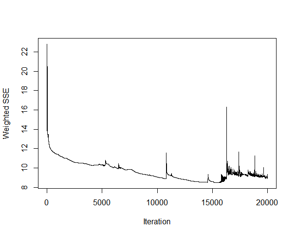
As you can see each training will give you different results.This iteration is based solely on the closing price!
> # Import the csv file
> quotes <- read.csv("E:/MarketData/EURUSD1440.csv", header=FALSE)
>
> tail(quotes)
             V1    V2      V3      V4      V5      V6     V7
2149 2016.05.25 00:00 1.11394 1.11670 1.11289 1.11552  99307
2150 2016.05.26 00:00 1.11545 1.12169 1.11494 1.11940 105208
2151 2016.05.27 00:00 1.11941 1.12008 1.11111 1.11131  97768
2152 2016.05.30 00:00 1.11142 1.11448 1.10980 1.11386  63587
2153 2016.05.31 00:00 1.11384 1.11729 1.11223 1.11317 111428
2154 2016.06.01 00:00 1.11316 1.11941 1.11142 1.11881 120272
>
> #number of rows in the dataframe
> x <-nrow(quotes)
>
> # load quantmod package
> library(quantmod)
>
> #convert the data frame into a ts object
> quotes <- as.ts(quotes)
>
> #convert time series into a zoo object
> quotes1 <- as.zoo(quotes)
>
>
> # lag the data
> x1 <- lag(quotes1, k=-1, na.pad=TRUE)
> x2 <- lag(quotes1, k=-2, na.pad=TRUE)
> x3 <- lag(quotes1, k=-3, na.pad=TRUE)
> x4 <- lag(quotes1, k=-4, na.pad=TRUE)
> x5 <- lag(quotes1, k=-5, na.pad=TRUE)
> x6 <- lag(quotes1, k=-6, na.pad=TRUE)
> x7 <- lag(quotes1, k=-7, na.pad=TRUE)
> x8 <- lag(quotes1, k=-8, na.pad=TRUE)
> x9 <- lag(quotes1, k=-9, na.pad=TRUE)
> x10 <-lag(quotes1, k=-10, na.pad=TRUE)
>
> #
> #Neural Network for the Close Price Time Series
> #
>
>
> # combine all the above matrices into one matrix having close prices
> CQuotes <- cbind (x1[,6], x2[,6], x3[,6], x4[,6], x5[,6],
+                   x6[,6], x7[,6], x8[,6], x9[,6], x10[,6],
+                   quotes1[,6])
>
> #scale the data
> CQuotes <- scale(CQuotes, center=T, scale=T)
>
> # create data for training
> inputs_trainC  <- CQuotes[15:x, 1:10]
> outputs_trainC <- CQuotes[15:x, 11]
>
> # load RSNNS package
> library(RSNNS)
>
> #build the Elman Neural Network
> modelC <- elman (inputs_trainC, outputs_trainC,
+                  size =c(15,15) ,
+                  learnFuncParams =c(0.1) ,
+                  maxit =20000)
>
> #build the Elman Neural Network
> modelC <- elman (inputs_trainC, outputs_trainC,
+                 size =c(15,15) ,
+                 learnFuncParams =c(0.1) ,
+                 maxit =20000)
>
>
>
> #make predictions
> predC <- predict(modelC , CQuotes[x, 1:10])
>
> CQuotes[x,11] <- predC[1]
> CQuotes[x+1, 1] <- predC[1]
>
> predC <- predict(modelC , CQuotes[x+1, 1:10])
>
> CQuotes[x+1,11] <- predC[1]
> CQuotes[x+2,2] <- CQuotes[x+1,1]
> CQuotes[x+2,1]  <- predC[1]
>
>
> predC <- predict(modelC , CQuotes[x+2, 1:10])
>
> CQuotes[x+2,11] <- predC[1]
> CQuotes[x+3,2] <- CQuotes[x+2,1]
> CQuotes[x+3,3] <- CQuotes[x+2,2]
> CQuotes[x+3,1]  <- predC[1]
>
>
> predC <- predict(modelC , CQuotes[x+3, 1:10])
>
> CQuotes[x+3,11] <- predC[1]
> CQuotes[x+4,2] <- CQuotes[x+3,1]
> CQuotes[x+4,3] <- CQuotes[x+3,2]
> CQuotes[x+4,4] <- CQuotes[x+3,3]
> CQuotes[x+4,1]  <- predC[1]
>
>
> predC <- predict(modelC , CQuotes[x+4, 1:10])
>
> CQuotes[x+4,11] <- predC[1]
>
> library(DMwR)
> predC1 <- unscale(CQuotes[(x):(x+4), 11], CQuotes)
>
> #closing price predictions
>
> predC1

2154 1.118340
2155 1.124287
2156 1.128586
2157 1.133033
2158 1.136264
> tail(quotes[,6])
[1] 1.11552 1.11940 1.11131 1.11386 1.11317 1.11881
As you can see from above, this time we only predicted the closing price as our model works best for the closing price. Our model is predicting the closing price for today to be 1.124287. The best approach would be to train the date 5-10 times on the closing price and then average the predicted price to remove outliers.If we want to calculate the daily high and low we need to remodel the inputs. We will try to use different inputs for the high and low and see if we get better results. The predicted results depend on our choice of inputs. Right now our Elman Neural Network is giving good results with the closing price with inputs as the lagged closing prices.
Did you read the post on USDCHF trade that made 61% return in 6 days? Naked trading is the best strategy. Just focus on price action. Each daily and weekly candle gives you important support and resistance levels that you should watch carefully. You should also read this post on a naked USDJPY trade that made 1000 pips.