In this post we are going to discuss in detail how we are going to use Random Forests algorithm in trading. The idea is to find an algorithm that can predict market movement over the next few hours which can be 5, 10, 15, 20, 25, 30 hours. If we can find such an algorithm we can increase our trading accuracy manifold. In this post we will try the Random Forests algorithm and see if we can use it to predict the market movement over the next few hours that can be 5 hours, 10 hours, 15 hours, 20 hours, 30 hours etc. We build a model that uses this algorithm to make the predictions. We then test this model and see if we have a good model and whether we can use it in actual trading.
Did you read our post on how to predict the daily candle using Elman Neural Network? Our objective is to find a algorithm that have more than 80% predictive accuracy. We then combine the predictions made by the algorithm with our manual trading strategy. This is done initially to test the algorithmic model. Once we have tested the algorithmic model thoroughly we can develop an EA based on it and us it as an automated trading system. Read the post on how to trade naked and make 1000 pips. Trading naked means trading without any indicators solely based on price action.
Efficient Market Hypothesis
Markets are highly complex and dynamic systems. Markets are highly interactive system that comprise of massive number of participants who are constantly changing their behavior due to news, politics and other outside stimuli. There is a feedback loop builtin that ensures that market continuously learns what the participants are doing and changes its behavior accordingly. Previously it was theorized that markets are efficient. Eugene Fama a finance professor had enunciated the Efficient Market Hypothesis. What this meant was that prices are efficient and all the available information immediately gets reflected in the price. There is no way that we can use past prices to predict future prices. Over the years this hypothesis got tested and it has been modified now.
Algorithmic Trading Is Also Known As Quantitative Trading
Today it is believed by researchers that markets are inefficient in the short term but efficient in the long run. It takes time for the information to get disseminated. This is the time when you can make a killing in the market by entering early and getting out at the right time. You can compare this statement with your technical analyst training. As technical traders we have been told to think ahead of the crowd and get in early before the trend matures and get out before the trend reverses. This is precisely what the new finance theory also enunciates. As new trend develops, information disseminates slowly. As information get disseminated, more people enter trades in the direction of the trend. This is how the trend continues. Then suddenly market gets a shock in the form of new news that reverses the trend. Read the post on how we made money trading gold.
A new subject known as Behavior Finance has been developed that explains the market behavior better than the traditional economics theory. Due to short term inefficiency it is possible to find patterns that can predict the short term behavior of the market. This is due to the slow dissemination of information as explained above. Once the information gets fully disseminated, markets become efficient and price reflects what is known to everyone by now.
Always keep this in mind when we are trading, we are always faced with uncertainty. Algorithmic trading has become very popular now a days. Algorithmic trading is also known as Quantitative trading. We use algorithm to find short term patterns in the market that can be used to make short term predictions. Keep this in mind that when we increase our predictive horizon, we lose our predictive accuracy. Shortest term predictions that are being made now a days is less than a second. This is known as high frequency trading. It has become very popular with hedge funds and high tech firms. Watch this documentary on high frequency trading.
What Is Random Forests Algorithm?
Random Forests is one of the popular, versatile and robust algorithm that is being used in making predictions in such diverse fields as health care, medicine, marketing, communications etc. Random Forests is basically an ensemble learning method. Ensemble learning means we will combine a few experts who are weak learners and try to make an expert who is a strong learner. Ensemble learning employs two methods that are known as bagging and boosting. Both these methods use bootstrap sampling to make numerous models that are then finally combined in a voting machine. Sounds complicated? We have posted 2 videos below which try to explain the Random Forests algorithm in detail.
You can think of Random Forests algorithm as a variant of Decision Trees algorithm. Basically it uses ensemble learning on decision trees. It uses bootstrap sampling and builds many trees. You can specify the number of trees that it should build before making the prediction. The problem with decision trees is that they are too much susceptible to noise and overfitting. Decision trees easily overfit data. A slight variation in data can produce an entirely different model. This problem gets minimized by Random Forests algorithm as it builds many decision trees and then uses the majority votes to make the decision. Below is an beginners guide to Random Forests algorithm.
In the above video, the speaker explains how she implemented Random Forests algorithm using Python language. Just as she had said Python is trying hard to overtake R as a the programming language of choice for data science and machine learning. Python is a pretty solid language that is 2-4 times faster than R. Eventually Python is going to supersede R as a language of choice for data science. R is based on a technology developed in the late 1950s. R is a bit slow and faces problems when the size of data sets become too large as it is very inefficient with memory. Python was developed in early 1990s and uses modern technology and can handle very large data sets efficiently.But we will do our analysis in R below. R has got an excellent technical analysis library that can make candlestick charts and calculate all sorts of technical indicators like the MACD, RSI, Aroon, Volatility, Stochastic, SAR, Bollinger Bands etc. Did you read the post on Aroon Indicator and how to trade with it.
Python still lacks a module that can do all these calculations. As long as some python developer doesn’t develop a module that does what Quantmod library in R does, we will be constrained to use R in our calculations. Maybe we develop this technical analysis module for Python in the future. But right now we lack this module in python and writing code for these technical indicators can be a laborious and time consuming process which can take months of testing. Below is another good video that tries to explain this algorithm in detail this time using R.
Now after watching the above videos you should be able to have a fair idea on how random forests algorithm works. Read the post on how to predict market reversals using daily and weekly candles. You should have R and RStudio installed on your computer. You should be familiar with R language. First we download the data from MT4 in a csv file. We download EURUSD 60 minutes data. We want to predict EURUSD price after 15 hours. We build a model to predict the closing price after 15 hours. We can change this time period using n variable in the code below. By changing n we can use this model to predict price after 2 hours, 5 hours, 10 hours, 15 hours, 20 hours, 30 hours etc. We add new columns to the data on RSI, MACD, CCI, William% R, Stochastic, Aroon and ATR etc.
Random Forest Predictive Model For Price
Our model will be able to predict whether price will move up and down with factors -3, -2, -1, 0, 1, 2, 3 and 4.Factors are categorical variables in R. 1 means price will move between 0 and 50 pip up. 2 mean price will move between 50 and 150 pip up. 3 means price will move between 150 and 300 pips up. 4 means price will move more than 300 pips up. Similarly -1 means price will move between 0 and 50 pip down. -2 means price will move between 50 and 150 pips down and -3 means price will move more than 300 pips down. Below is the code and its run results:
> ###Random Forest Classification Strategy Back Test###
> #import the data
>
> data <- read.csv("E:/MarketData/EURUSD60.csv", header = FALSE)
>
>
>
> colnames(data) <- c("Date", "Time", "Open", "High",
+                     "Low", "Close", "Volume")
>
>
> x1 <- nrow(data)
>
> #convert this data to n timeframe
>
> n=15
>
> #define lookback
>
> lb=500
>
> #define the minimum pips
>
> pip <- 50
>
> #define a new data frame
>
> data1 <-data.frame(matrix(0, ncol=6, nrow=300))
>
> colnames(data1) <- c("Date", "Time", "Open", "High",
+                      "Low", "Close")
>
> # run the sequence to convert to a new timeframe
>
> for ( k in (1:lb))
+ {
+   data1[k,1] <- as.character(data[x1-lb*n+n*k-1,1])
+   data1[k,2] <- as.character(data[x1-lb*n+n*k-1,2])
+   data1[k,3] <- data[x1-lb*n+n*(k-1),3]
+   data1[k,6] <- data[x1-lb*n+n*k-1,6]
+   data1[k,4] <- max(data[(x1-lb*n+n*(k-1)):(x1-lb*n+k*n-1), 4:5])
+   data1[k,5] <- min(data[(x1-lb*n+n*(k-1)):(x1-lb*n+k*n-1), 4:5])
+ }
>
>
> library(quantmod)
>
> data2 <- as.xts(data1[,-(1:2)], as.POSIXct(paste(data1[,1],data1[,2]),
+                                            format='%Y.%m.%d %H:%M'))
>
>
>
> data2$rsi <- RSI(data2$Close)
> data2$MACD <- MACD(data2$Close)
> data2$will <- williamsAD(data2[,2:4])
> data2$cci <-  CCI(data2[,2:4])
> data2$STOCH <- stoch(data2[,2:4])
> data2$Aroon <- aroon(data2[, 2:3])
> data2$ATR <- ATR(data2[, 2:4])
>
>
> data2$Return <- diff(log(data2$Close))
>
>
>
> candleChart(data2[,(1:4)],
+             theme='white', type='candles', subset='last 10 days')
>
>
> for (i in (1:(lb-1)))
+ {
+
+   data2[i,20] <- data2[i+1,20]
+
+
+ }
>
> data3 <- as.data.frame(data2)
>
> #convert return into factors
>
> rr1 <- (pip/10000)/data1[lb, 6]
> rr2 <- 3*(pip/10000)/data1[lb, 6]
> rr3 <- 6*(pip/10000)/data1[lb, 6]
>
> # convert the returns into factors
>
> nn <- ncol(data3)
>
> data3$Direction <- ifelse(data3[ ,nn] > rr3, 4,
+                           ifelse(data3[ ,nn] > rr2, 3,
+                                  ifelse(data3[ ,nn] > rr1, 2,
+                                         ifelse(data3[ ,nn] > 0, 1,
+                                                ifelse(data3[ ,nn] > -rr1, -1,
+                                                       ifelse(data3[ ,nn] > -rr2, -2,
+                                                              ifelse(data3[ ,nn] > -rr3,  -3, -3)))))))
>
>
>
>
> data3 <- data3[,-nn]
>
> data3$Direction <- factor(data3$Direction)
>
> str(data3)
'data.frame':	500 obs. of  20 variables:
 $ Open     : num  1.11 1.11 1.12 1.11 1.12 ...
 $ High     : num  1.11 1.12 1.12 1.12 1.12 ...
 $ Low      : num  1.1 1.11 1.11 1.11 1.11 ...
 $ Close    : num  1.11 1.12 1.11 1.12 1.11 ...
 $ rsi      : num  NA NA NA NA NA NA NA NA NA NA ...
 $ macd     : num  NA NA NA NA NA NA NA NA NA NA ...
 $ MACD     : num  NA NA NA NA NA NA NA NA NA NA ...
 $ will     : num  NA 0.01123 0.00438 0.0124 0.00446 ...
 $ cci      : num  NA NA NA NA NA NA NA NA NA NA ...
 $ fastK    : num  NA NA NA NA NA NA NA NA NA NA ...
 $ fastD    : num  NA NA NA NA NA NA NA NA NA NA ...
 $ STOCH    : num  NA NA NA NA NA NA NA NA NA NA ...
 $ aroonUp  : num  NA NA NA NA NA NA NA NA NA NA ...
 $ aroonDn  : num  NA NA NA NA NA NA NA NA NA NA ...
 $ Aroon    : num  NA NA NA NA NA NA NA NA NA NA ...
 $ tr       : num  NA 0.0157 0.00818 0.00858 0.0091 ...
 $ atr      : num  NA NA NA NA NA NA NA NA NA NA ...
 $ trueHigh : num  NA 1.12 1.12 1.12 1.12 ...
 $ ATR      : num  NA 1.11 1.11 1.11 1.11 ...
 $ Direction: Factor w/ 7 levels "-3","-2","-1",..: 5 3 4 3 3 3 3 4 5 4 ...
>
> #load the randomForest library
>
>
> library ("randomForest")
>
> #define number of trees that randomForest will built
>
> num.trees =1000
>
>
>
> # train a randomForest Model
>
> formula("Direction ~ rsi+macd+MACD+will+cci+fastK+fastD+
+         STOCH+aroonUp+aroonDn+Aroon+
+         tr+ atr+ trueHigh+ATR")
Direction ~ rsi + macd + MACD + will + cci + fastK + fastD +
    STOCH + aroonUp + aroonDn + Aroon + tr + atr + trueHigh +
    ATR
>
> fit <- randomForest(Direction~., data=data3[100:(lb-1),1:nn],
+                     ntree = num.trees , importance =TRUE,
+                     proximity =TRUE )
> #print the model details
> print(fit)

Call:
 randomForest(formula = Direction ~ ., data = data3[100:(lb -      1), 1:nn], ntree = num.trees, importance = TRUE, proximity = TRUE)
               Type of random forest: classification
                     Number of trees: 1000
No. of variables tried at each split: 4

        OOB estimate of  error rate: 61%
Confusion matrix:
   -3 -2 -1  1 2 3 4 class.error
-3  0  0  0  1 0 0 0   1.0000000
-2  0  2 22 12 1 0 0   0.9459459
-1  0  1 88 75 4 0 0   0.4761905
1   0  3 85 66 2 0 0   0.5769231
2   0  1 18 15 0 0 0   1.0000000
3   0  0  0  3 0 0 0   1.0000000
4   0  0  1  0 0 0 0   1.0000000
>
> #plot the model
> plot(fit)
>
> ## predict the next candle size
> pred <-predict (fit , newdata =data3[lb, 1:(nn-1)], type ="class")
> pred
2016-10-25 10:00:00
                 -1
Levels: -3 -2 -1 1 2 3 4
>
> ## predict the probability of each class
> pred <-predict(fit , newdata =data3[lb, 1:(nn-1)], type ="prob")
> pred
                    -3    -2    -1     1     2     3     4
2016-10-25 10:00:00  0 0.052 0.592 0.292 0.046 0.017 0.001
attr(,"class")
[1] "matrix" "votes"
>
> data1[lb,2]
[1] "10:00"
> data1[lb,6]
[1] 1.08752
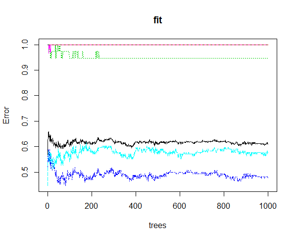
In the above results you can see that this Random Forest algorithm has also printed the confusion matrix that shows how many predictions were correct and how many predictions were wrong. It also prints the OOB (out of bag) error which is 61%. What this means is that our model is only 39% accurate in making predictions. The prediction made by our Random Forest model is -1 which means price will be between 0 and 50 pips below the present closing price after 15 hours. Present closing price is 1.08752 and the closing price after 15 hours was 1.08900. So the price closed 15 pips above the closing price after 15 hours. Our model had predicted the price to be between 0 and 50 pips below the present closing price. So the prediction was wrong. Watch videos on Inside Bar Trading Strategy. Below is the fit error plot of this model.
Improving The Random Forest Price Prediction Model Accuracy
So how do we improve the performance and accuracy of our model? You can try different mtry. In the above model the default mtry of 4 was used. We can change the default split using this mtry parameter This variable selects the number of features from the dataframe. Instead we add more technical indicators that includes the Bollinger Bands, Stochastic Momentum Index, Chaikin Volatility indicator as well as the Volatility indicator and the Close Location Value Indicator. Let’s try again now and see how well the model performs.
> ###Random Forest Classification###
> #import the data
>
> data <- read.csv("E:/MarketData/EURUSD60.csv", header = FALSE)
>
>
>
> colnames(data) <- c("Date", "Time", "Open", "High",
+                     "Low", "Close", "Volume")
>
>
> x1 <- nrow(data)
>
>
> #convert this data to n timeframe
>
> n=15
>
> #define lookback
>
> lb=500
>
> #define the minimum pips
>
> pip <- 50
>
> #define a new data frame
>
> data1 <-data.frame(matrix(0, ncol=6, nrow=300))
>
> colnames(data1) <- c("Date", "Time", "Open", "High",
+                      "Low", "Close")
>
> # run the sequence to convert to a new timeframe
>
> for ( k in (1:lb))
+ {
+   data1[k,1] <- as.character(data[x1-lb*n+n*k-1,1])
+   data1[k,2] <- as.character(data[x1-lb*n+n*k-1,2])
+   data1[k,3] <- data[x1-lb*n+n*(k-1),3]
+   data1[k,6] <- data[x1-lb*n+n*k-1,6]
+   data1[k,4] <- max(data[(x1-lb*n+n*(k-1)):(x1-lb*n+k*n-1), 4:5])
+   data1[k,5] <- min(data[(x1-lb*n+n*(k-1)):(x1-lb*n+k*n-1), 4:5])
+ }
>
>
> library(quantmod)
>
> data2 <- as.xts(data1[,-(1:2)], as.POSIXct(paste(data1[,1],data1[,2]),
+                                            format='%Y.%m.%d %H:%M'))
>
>
>
> data2$rsi <- RSI(data2$Close)
> data2$MACD <- MACD(data2$Close)
> data2$will <- williamsAD(data2[,2:4])
> data2$cci <-  CCI(data2[,2:4])
> data2$STOCH <- stoch(data2[,2:4])
> data2$Aroon <- aroon(data2[, 2:3])
> data2$ATR <- ATR(data2[, 2:4])
> data2$SMI <- SMI(data2[, 2:4])
> data2$BB <- BBands(data2[, 2:4])
> data2$ChaikinVol <-Delt(chaikinVolatility(data2[, 2:3]))
> data2$CLV <- EMA(CLV(data2[, 2:4]))
> data2$Volatility <- volatility(data2[, 1:4], calc="garman")
>
>
> data2$Return <- diff(log(data2$Close))
>
>
>
> candleChart(data2[,1:4],
+             theme='white', type='candles', subset='last 7 days')
>
>
>
> for (i in (1:(lb-1)))
+ {
+
+   data2[i,20] <- data2[i+1,20]
+
+
+ }
>
> data3 <- as.data.frame(data2)
>
> #convert return into factors
>
> rr1 <- (pip/10000)/data1[lb, 6]
> rr2 <- 3*(pip/10000)/data1[lb, 6]
> rr3 <- 6*(pip/10000)/data1[lb, 6]
>
> # convert the returns into factors
>
> nn <- ncol(data3)
>
> data3$Direction <- ifelse(data3[ ,nn] > rr3, 4,
+                           ifelse(data3[ ,nn] > rr2, 3,
+                                  ifelse(data3[ ,nn] > rr1, 2,
+                                         ifelse(data3[ ,nn] > 0, 1,
+                                                ifelse(data3[ ,nn] > -rr1, -1,
+                                                       ifelse(data3[ ,nn] > -rr2, -2,
+                                                              ifelse(data3[ ,nn] > -rr3,  -3, -3)))))))
>
>
>
>
> data3 <- data3[,-nn]
>
> data3$Direction <- factor(data3$Direction)
>
> str(data3)
'data.frame':	500 obs. of  29 variables:
 $ Open      : num  1.11 1.11 1.12 1.11 1.12 ...
 $ High      : num  1.11 1.12 1.12 1.12 1.12 ...
 $ Low       : num  1.1 1.11 1.11 1.11 1.11 ...
 $ Close     : num  1.11 1.12 1.11 1.12 1.11 ...
 $ rsi       : num  NA NA NA NA NA NA NA NA NA NA ...
 $ macd      : num  NA NA NA NA NA NA NA NA NA NA ...
 $ MACD      : num  NA NA NA NA NA NA NA NA NA NA ...
 $ will      : num  NA 0.01123 0.00438 0.0124 0.00446 ...
 $ cci       : num  NA NA NA NA NA NA NA NA NA NA ...
 $ fastK     : num  NA NA NA NA NA NA NA NA NA NA ...
 $ fastD     : num  NA NA NA NA NA NA NA NA NA NA ...
 $ STOCH     : num  NA NA NA NA NA NA NA NA NA NA ...
 $ aroonUp   : num  NA NA NA NA NA NA NA NA NA NA ...
 $ aroonDn   : num  NA NA NA NA NA NA NA NA NA NA ...
 $ Aroon     : num  NA NA NA NA NA NA NA NA NA NA ...
 $ tr        : num  NA 0.0157 0.00818 0.00858 0.0091 ...
 $ atr       : num  NA NA NA NA NA NA NA NA NA NA ...
 $ trueHigh  : num  NA 1.12 1.12 1.12 1.12 ...
 $ ATR       : num  NA 1.11 1.11 1.11 1.11 ...
 $ SMI       : num  NA NA NA NA NA NA NA NA NA NA ...
 $ SMI.1     : num  NA NA NA NA NA NA NA NA NA NA ...
 $ dn        : num  NA NA NA NA NA NA NA NA NA NA ...
 $ mavg      : num  NA NA NA NA NA NA NA NA NA NA ...
 $ up        : num  NA NA NA NA NA NA NA NA NA NA ...
 $ BB        : num  NA NA NA NA NA NA NA NA NA NA ...
 $ ChaikinVol: num  NA NA NA NA NA NA NA NA NA NA ...
 $ CLV       : num  NA NA NA NA NA ...
 $ Volatility: num  NA NA NA NA NA ...
 $ Direction : Factor w/ 7 levels "-3","-2","-1",..: NA 5 3 4 3 3 3 3 4 5 ...
>
> #load the randomForest library
>
>
> library ("randomForest")
>
> #define number of trees that randomForest will built
>
> num.trees =1000
>
>
>
> # train a randomForest Model
>
>
> fit <- randomForest(Direction~., data=data3[100:(lb-1),1:nn],
+                     ntree = num.trees , importance =TRUE,
+                     proximity =TRUE )
> #print the model details
> print(fit)

Call:
 randomForest(formula = Direction ~ ., data = data3[100:(lb -      1), 1:nn], ntree = num.trees, importance = TRUE, proximity = TRUE)
               Type of random forest: classification
                     Number of trees: 1000
No. of variables tried at each split: 5

        OOB estimate of  error rate: 44%
Confusion matrix:
   -3 -2  -1   1  2 3 4 class.error
-3  0  0   1   0  0 0 0   1.0000000
-2  0  7  22   5  3 0 0   0.8108108
-1  0  5 107  53  2 0 0   0.3592814
1   0  2  49 100  6 0 0   0.3630573
2   0  0   5  19 10 0 0   0.7058824
3   0  0   0   1  2 0 0   1.0000000
4   0  0   0   0  1 0 0   1.0000000
>
> #plot the model
> plot(fit)
>
> ## predict the next candle size
> pred <-predict (fit , newdata =data3[lb, 1:(nn-1)], type ="class")
> pred
2016-10-25 10:00:00
                  1
Levels: -3 -2 -1 1 2 3 4
>
> ## predict the probability of each class
> pred <-predict(fit , newdata =data3[lb, 1:(nn-1)], type ="prob")
> pred
                    -3    -2    -1     1     2 3 4
2016-10-25 10:00:00  0 0.016 0.487 0.496 0.001 0 0
attr(,"class")
[1] "matrix" "votes"
>
> data1[lb,2]
[1] "10:00"
> data1[lb,6]
[1] 1.08752
Did you see, this time the prediction was 1. Yes it was 1. Our model made the correct prediction this time. Price was predicted to move up between 0 and 50 pips and indeed it did move up by 15 pips. We have also succeeded in improving the predictive accuracy of the model. This time OOB (out off bag) error has been reduced to 44% meaning our model has now a predictive accuracy of 56%. We can work more on this model and try to reduce the error to below 20%. If we can do that our model will have a predictive accuracy of 80%. Once we can predict the price with 80% accuracy this will improve our trading results. Before entering into a trade, we use our model to check how much the price is going to move and in which direction. This will help us in avoiding opening a trade in the wrong direction. Read the post on a swing trade that made 100% in 24 hours.